PortBench

A Correlation-Aware, Full-Pipeline Benchmark
for LLM-Driven Portfolio Management


1Yantai Research Institute of Harbin Engineering University   2The Hong Kong University of Science and Technology (Guangzhou)

Corresponding to: sijiachen@hkust-gz.edu.cn
PortBench overview

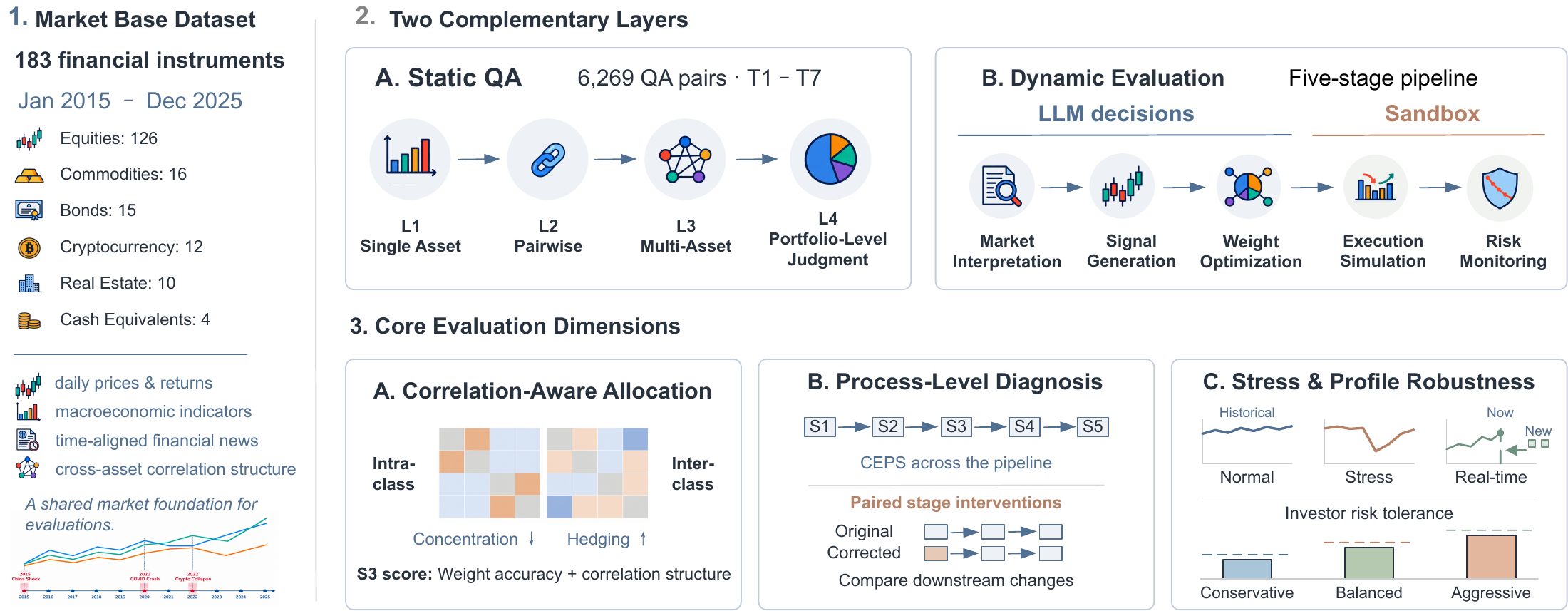
Overview of PortBench. We first collect the Market Base Dataset (183 instruments Γ— 6 asset classes, 2015–2025), then build a dual-layer evaluation framework on top: a static QA layer (6,269 correlation-based pairs) and a dynamic five-stage pipeline, jointly assessed under three risk profiles and three historical stress regimes.

Introduction

Large language models (LLMs) have shown strong performance across diverse financial tasks, yet portfolio management (PM), a critical financial decision-making task, remains poorly benchmarked. Existing benchmarks exhibit two main gaps: they ignore cross-asset correlation structures, failing to distinguish genuinely diversified portfolios from concentrated ones, and fail to evaluate the complete PM decision pipeline in real-world scenarios.

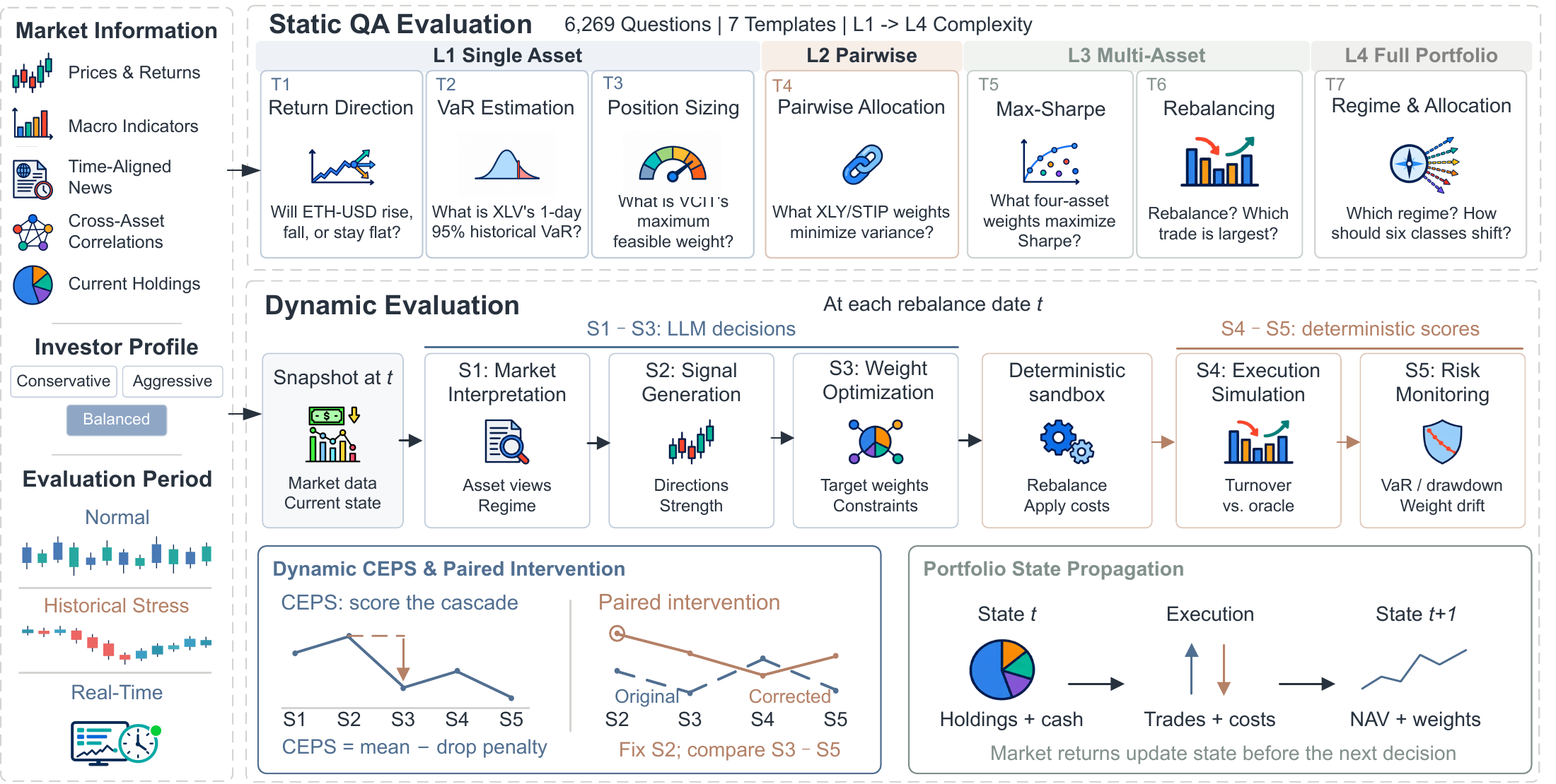
We introduce PortBench, a benchmark spanning six heterogeneous asset classes over ten years. PortBench consists of two complementary layers: a static QA dataset of 6,269 correlation-based questions across seven task templates, and a dynamic five-stage allocation pipeline that mirrors the full PM decision cycle. To evaluate these layers we introduce two dedicated metrics: a dual-layer correlation score that measures whether proposed portfolios exploit inter-class hedging and avoid intra-class concentration, and CEPS, which quantifies how reasoning errors compound across pipeline stages. We further assess strategy robustness and investor alignment under three historical stress regimes and three risk profiles.

Critically, every component of PortBench is objective, traceable, and scalable. The framework rests on a single auditable source: the Market Base Dataset. QA pairs are auto-generated via rule-based templates without human annotation, enabling seamless extension to new periods and assets. Crucially, pipeline ground truths are validated strictly against realized future returns that are withheld from LLM prompts (ensuring point-in-time safety). Thus, every S1–S5 score traces back to observed market outcomes, free from human judgment, oracle leakage, or hidden assumptions. This guarantees fair, reproducible comparisons and allows the benchmark to scale without manual re-annotation.

Evaluating ten frontier LLMs, we find that despite strong performance on static financial QA, 90% of model-profile combinations fail to outperform a basic equal-weight allocation, and models that satisfy every procedural constraint still suffer catastrophic drawdowns under stress.

Evaluation framework

Evaluation framework. Static QA layer (Top): seven task templates generated automatically from historical data. Dynamic five-stage pipeline (Bottom): executed sequentially at every rebalance date under three investor profiles and three stress regimes.

PortBench Explorer

The sections below let you interactively explore each layer of the PortBench framework. Start with the raw Market Base Dataset, then dive into the two evaluation layers that run on top of it.

Market Base Dataset

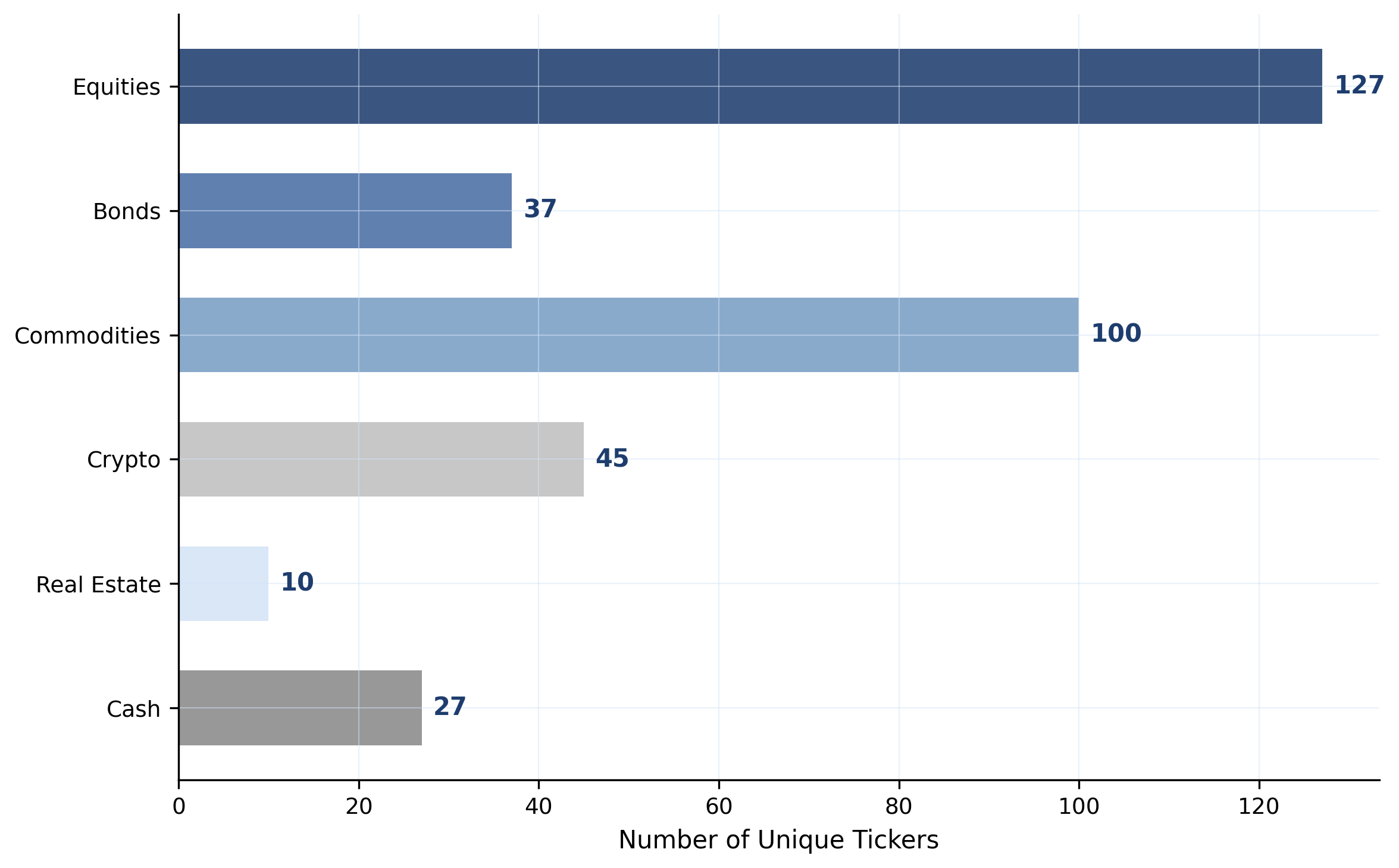
The Market Base Dataset covers 183 unique financial instruments spanning 2015–2025 across six heterogeneous asset classes, collected from Yahoo Finance, FRED, and Kaggle. Equities exhibit the broadest coverage (126 tickers), reflecting the diversity of broad-market, sector, and factor ETFs. Commodities (16) and bonds (15) provide representative cross-class hedging opportunities; cryptocurrency (12) captures major and mid-cap digital assets; real estate (10) and cash equivalents (4) round out the defensive allocation universe.

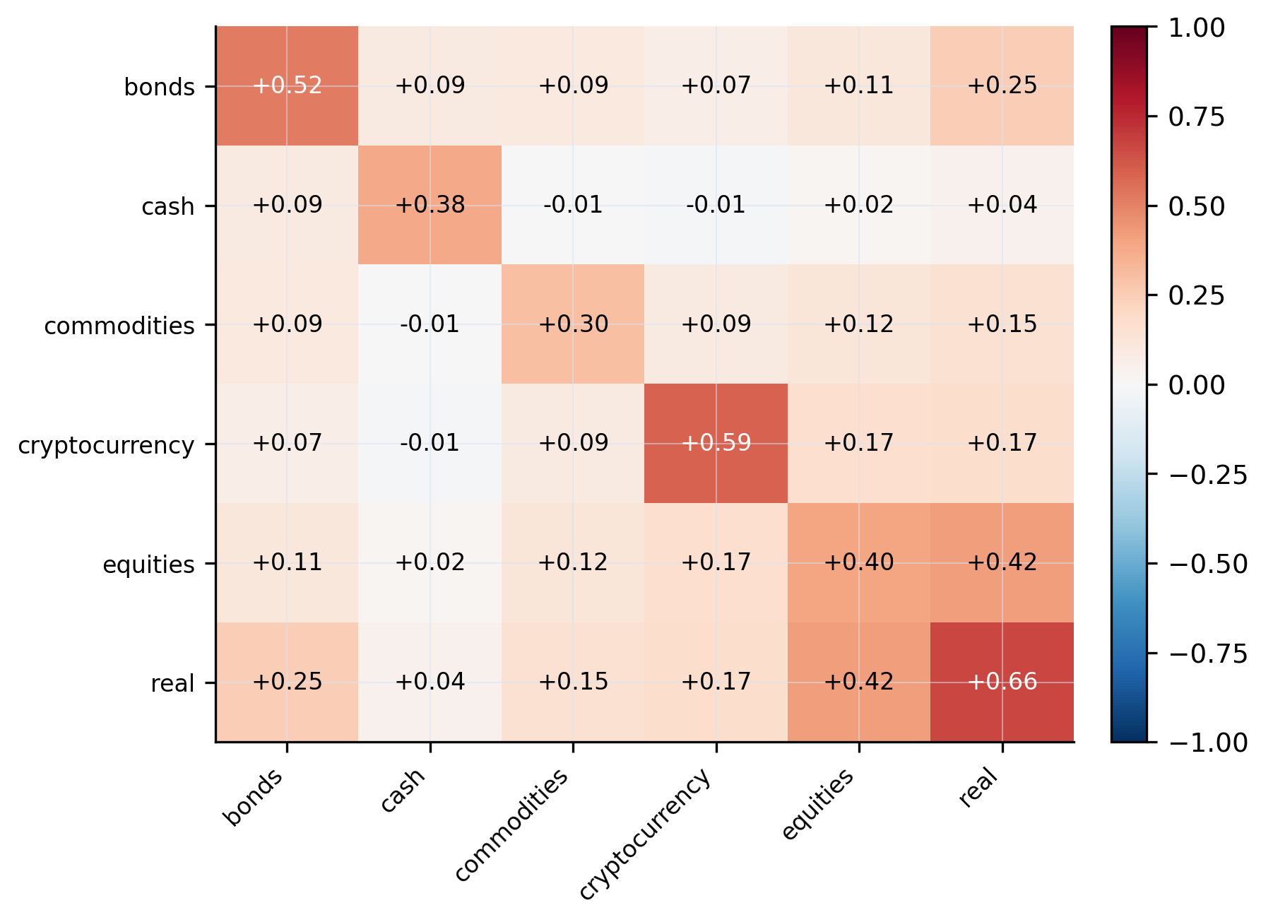
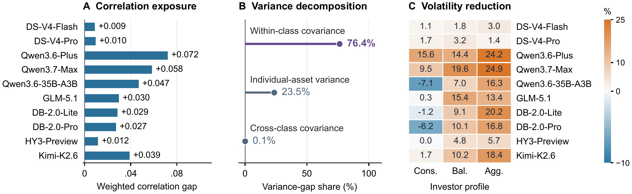
Correlation analysis reveals that inter-class average correlations are generally low while intra-class correlations are strongly positive. True diversification requires crossing asset class boundaries, not merely spreading across tickers within the same class, directly motivating the two-layer correlation scoring design.

Interactive Market Snapshot

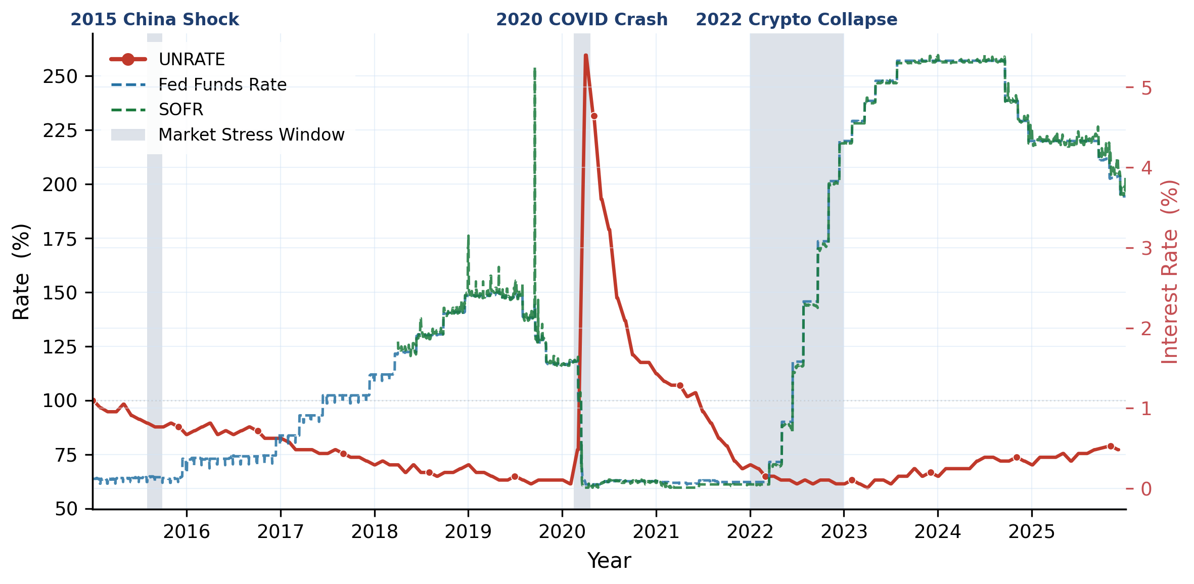
183 instruments across 6 asset classes, daily data 2015–2025. Each monthly snapshot includes macro indicators, per-asset price summaries, and cross-class correlations. Select a date to see the full snapshot.

Loading market data…
Instrument count by asset class

Number of unique tickers/series per asset class.

Correlation matrix

Pairwise Pearson correlation matrix (daily returns, 2015–2022).

Inter-class correlation

Mean pairwise correlation: each class vs. all others.

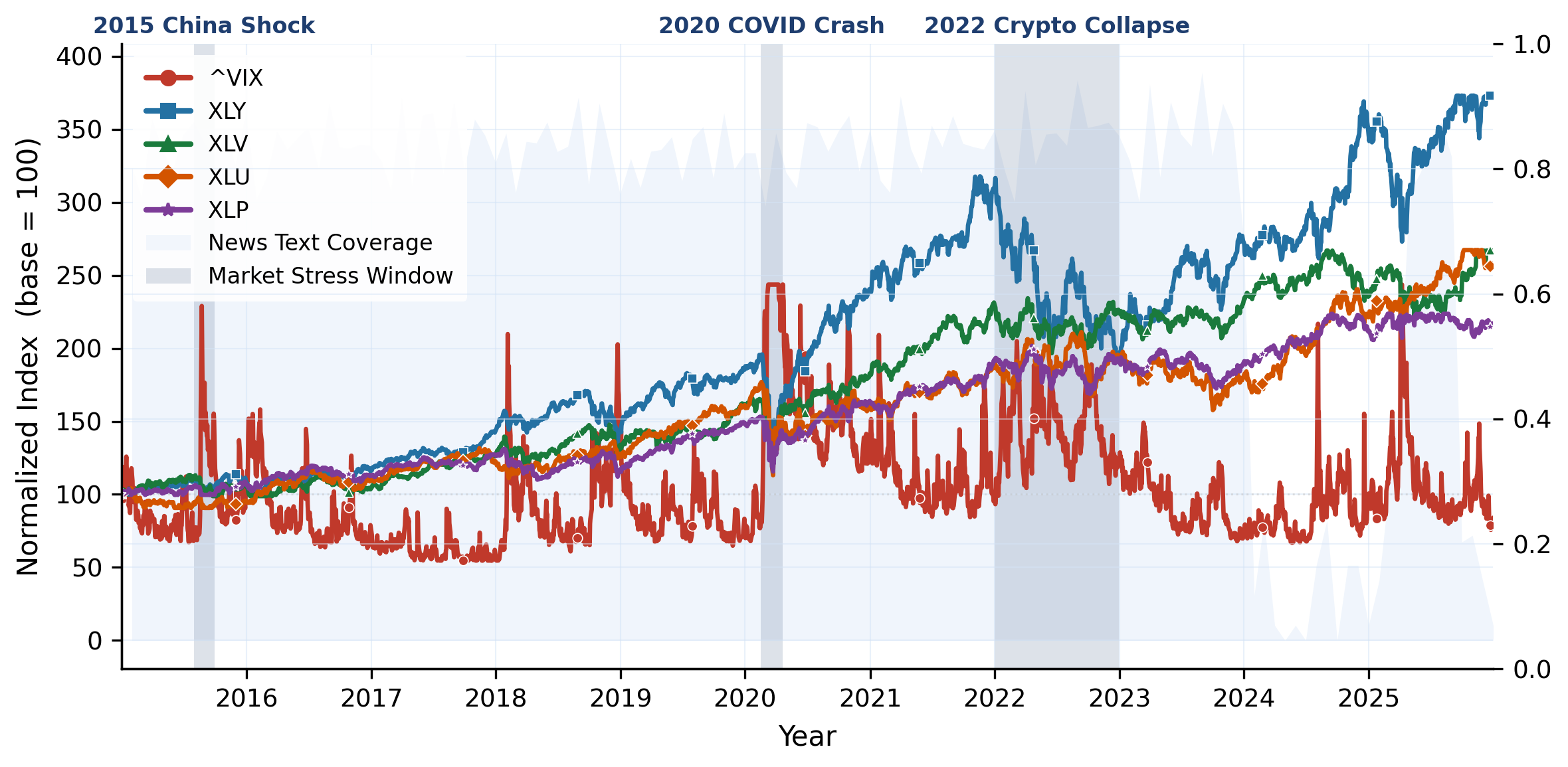
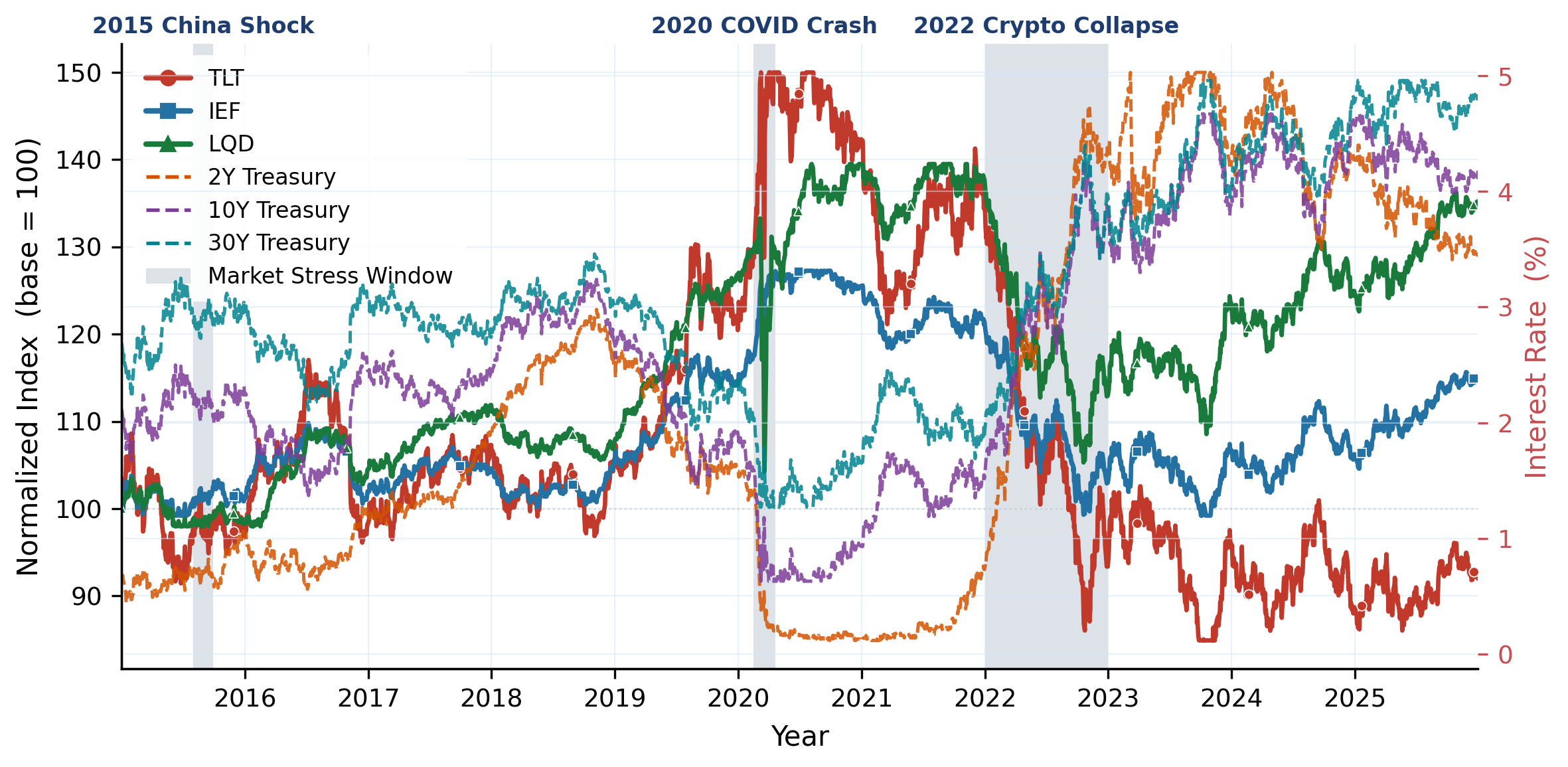
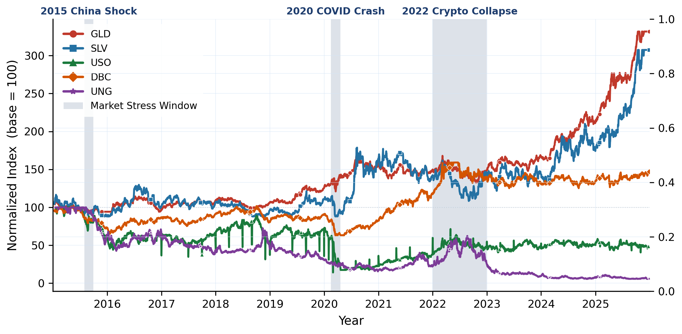
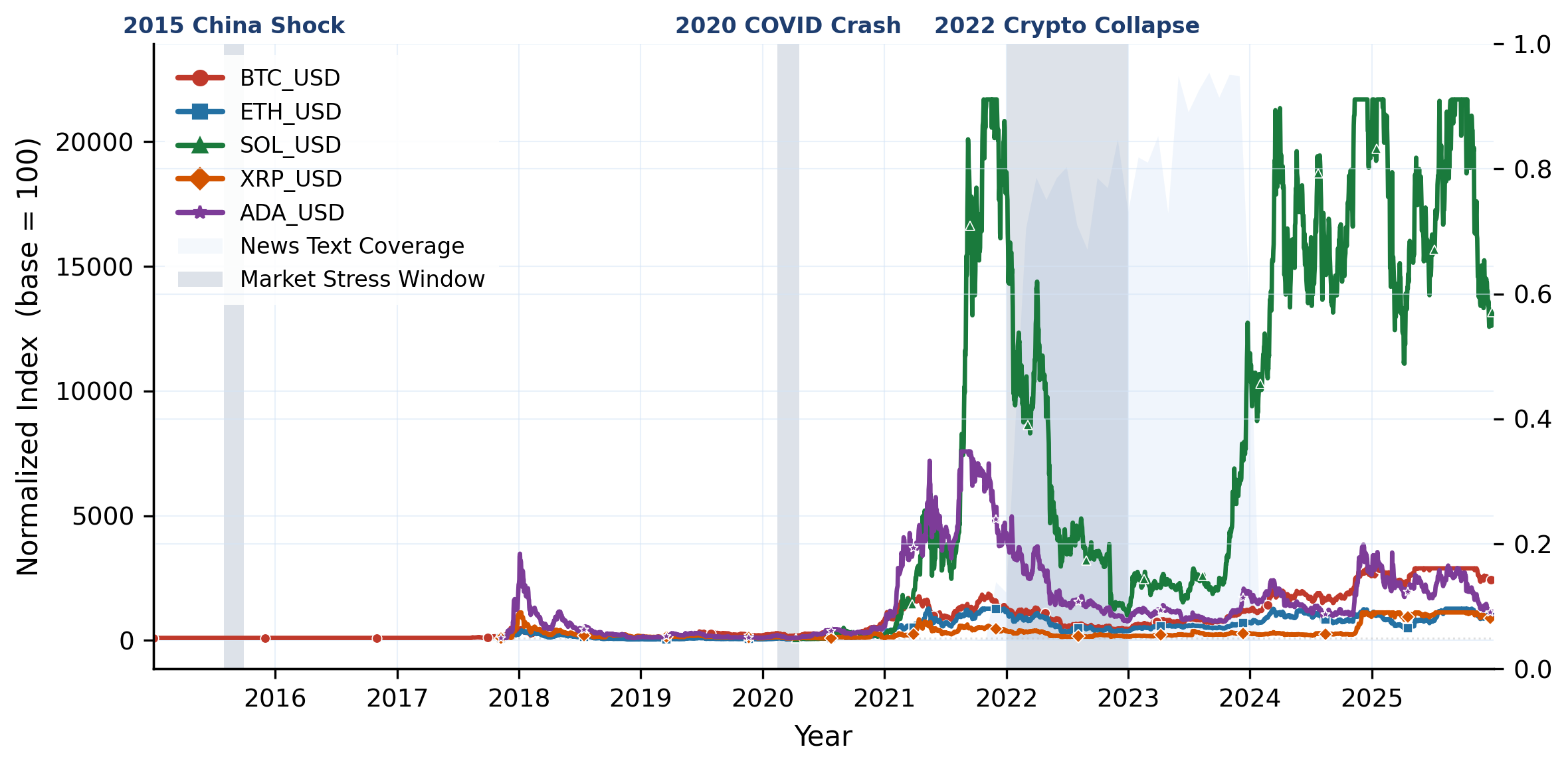
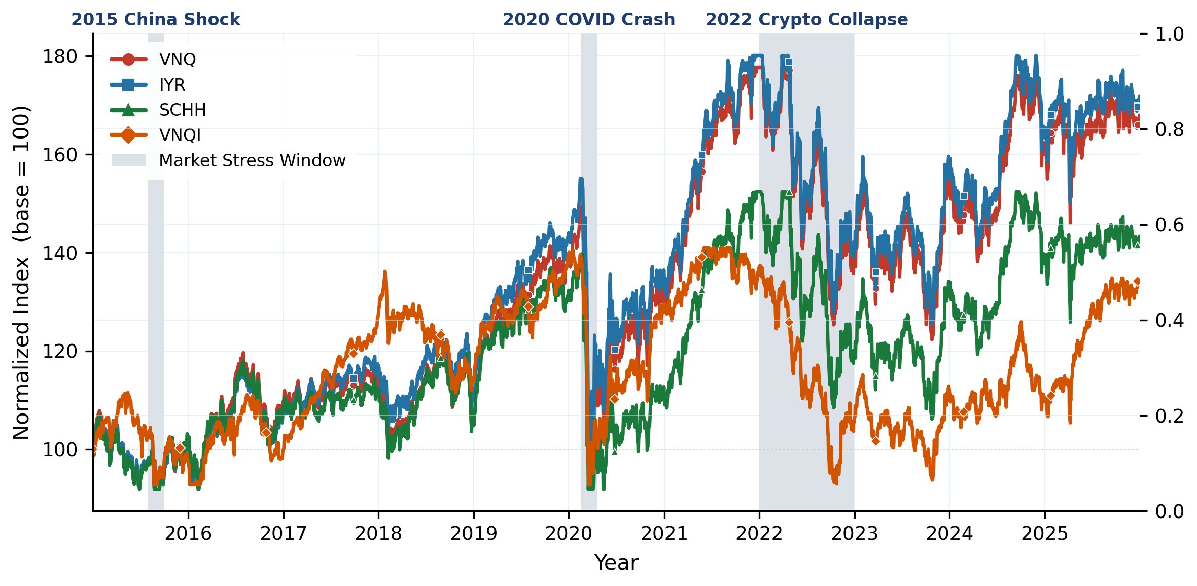
Normalized Price Trajectories by Asset Class (2015–2025)

Base = 100 at first listing date. Each panel shows representative instruments from one asset class.

Evaluation Framework

The evaluation framework has two complementary layers. Switch between the tabs below to explore the QA Dataset and the Pipeline Evaluation in detail.

6,269 correlation-aware QA pairs across 7 task templates (T1–T7), spanning complexity levels 1–4 and three market regimes. Select a template to browse sample question–answer pairs.

Evaluation Details

At a Glance

10
LLMs Evaluated
5
Classical Baselines
6
Asset Classes
183
Financial Instruments
6,269
QA Pairs
10 yr
2015 – 2025

Five-Stage Decision Pipeline

At each rebalance date the LLM executes S1–S5 sequentially. LLMs and classical baselines share the identical backtest environment for controlled comparison.


S1 Β· Market Interpretation Continuous sentiment views vi ∈ [βˆ’1,+1] per asset. Scored as 1 βˆ’ MAE(views, ground-truth) / 2.
S2 Β· Signal Generation Views discretized into buy / hold / sell signals (thresholds Β±0.2). Scored as fraction of assets with the correct direction.
S3 Β· Weight Optimization Portfolio weights scored by the two-layer correlation score: weight accuracy (L₁ to signal-constrained max-Sharpe optimum, Ξ± = 0.5) + correlation structure (intra-class concentration penalty + inter-class hedging credit). Ground truth computed from realized future returns with strict PiT safety.
S4 Β· Execution Simulation Deterministic. Fixed transaction costs (10 bps slippage + 5 bps commission). Scores turnover deviation from the oracle rebalancing rate.
S5 Β· Risk Monitoring Deterministic. 50% rebalance-trigger accuracy + 50% VaR/drawdown estimation accuracy. Rebalance trigger fires when max single-asset drift exceeds 5%.

CEPS: Cross-Stage Error Propagation Score

Prior benchmarks obscure early reasoning failures by averaging scores. CEPS penalizes error cascades, a strong stage followed by a weak one, more heavily than uniform mediocrity, capturing the operational reality that a perfectly interpreted market view is worthless if signal generation immediately fails.

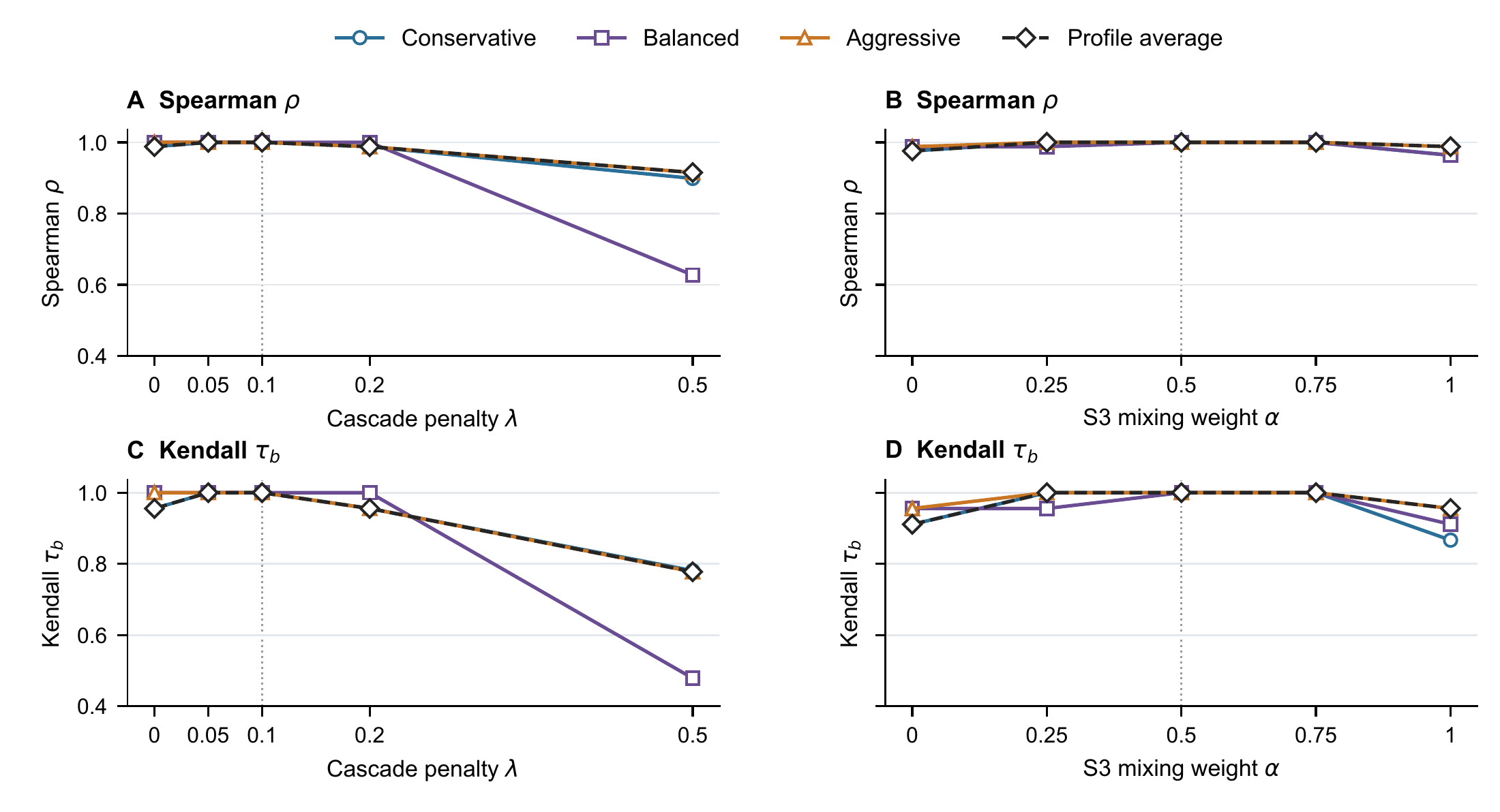
CEPS = clip( mean(σ₁…σ₅) βˆ’ Ξ» Β· Ξ£ max(Οƒβ‚œ βˆ’ Οƒβ‚œβ‚Šβ‚, 0), 0, 1 ) Default propagation weight Ξ» = 0.1

Ground truth for all LLM-scored stages is derived from realized future returns withheld from prompts, guaranteeing point-in-time (PiT) safety throughout.

CEPS: Cascade vs. Uniform Mediocrity

Two models with identical average stage scores (0.526) receive different CEPS scores because one cascades errors while the other is uniformly mediocre.

S1S2S3S4S5Avg
Model A (cascade)0.7920.5060.7140.1360.4800.526
Model B (uniform)0.5260.5260.5260.5260.5260.526
Model A (cascade)Model B (uniform)
Isolated avg0.5260.526
Cascade drops(0.792-0.506) + (0.714-0.136) = 0.286 + 0.578 = 0.8640
Penalty (lambda=0.1)0.1 x 0.864 = 0.0860
CEPS0.526 - 0.086 = 0.4400.526 - 0 = 0.526
The cascade penalty (lambda=0.1) reduces Model A's CEPS by 0.086, penalizing the sharp S1 to S2 and S3 to S4 drops that indicate brittle error propagation. Model B's uniform mediocrity incurs no penalty.

Investor Profiles & Stress Regimes

CEPS is evaluated under three investor risk profiles with escalating risk tolerance, and back-tested across three historical stress regimes to assess robustness when market conditions deteriorate sharply.

πŸ›‘οΈ
Conservative
Equity + Crypto≀ 40%
Bond + Cashβ‰₯ 40%
Max Drawdown≀ 10%
Daily VaR (95%)≀ βˆ’1.0%
βš–οΈ
Balanced
Equity + Crypto≀ 65%
Bond + Cashβ‰₯ 20%
Max Drawdown≀ 20%
Daily VaR (95%)≀ βˆ’2.0%
πŸš€
Aggressive
Equity + Crypto≀ 90%
Bond + Cashβ‰₯ 5%
Max Drawdown≀ 35%
Daily VaR (95%)≀ βˆ’4.0%

Each profile is tested under three historical stress regimes:

2015
China Shock
Aug 2015 – Feb 2016
liquidity-driven
2020
COVID Crash
Feb 2020 – May 2020
pandemic-driven
2022
Crypto Collapse
May 2022 – Dec 2022
monetary-tightening-driven

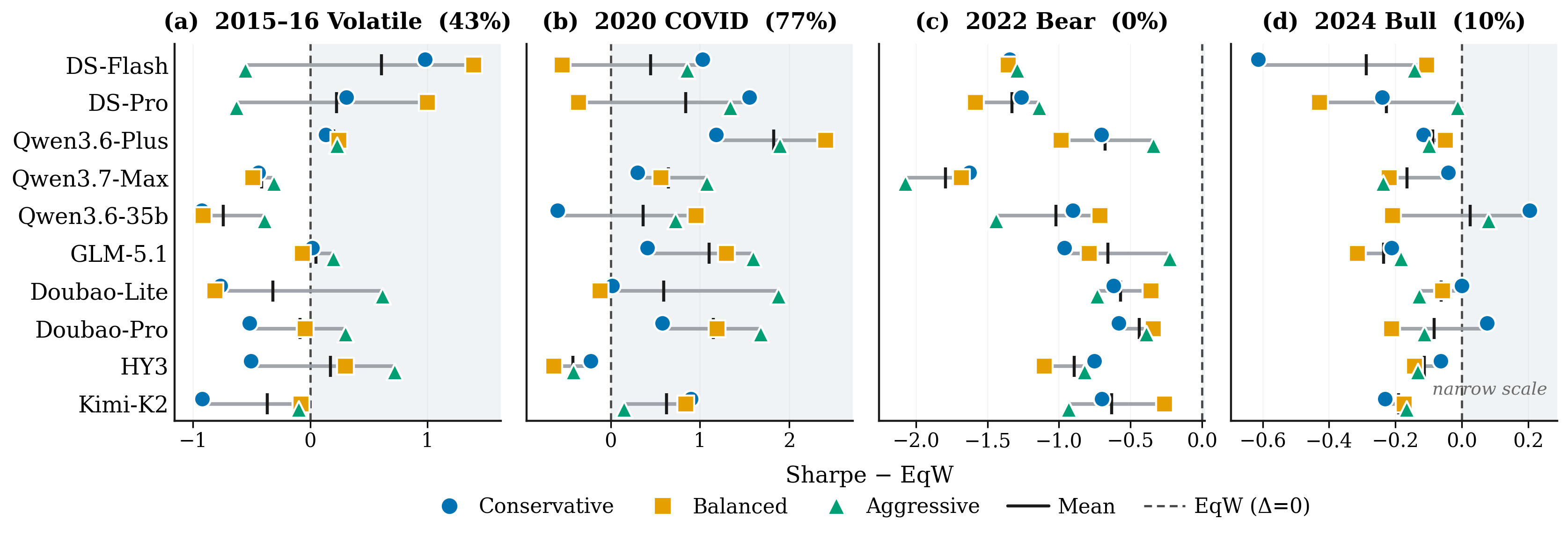
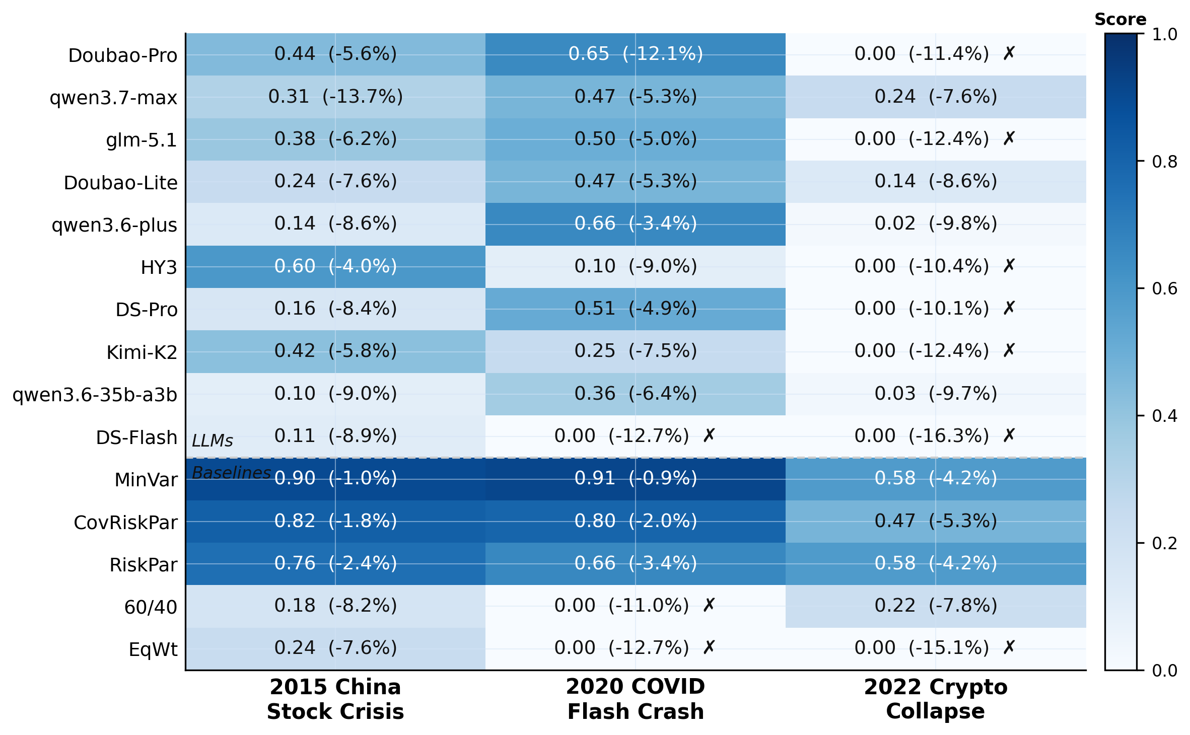
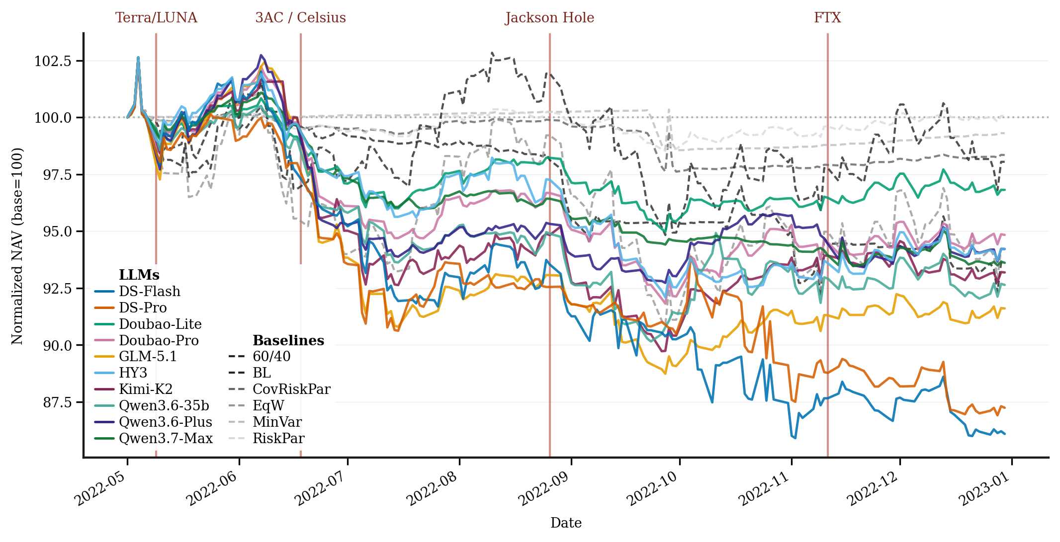
A model passes the stress gate for a given profile if its maximum drawdown across all three regimes stays within the profile's tolerance. Six of ten models fail the Conservative stress gate, all during the 2022 Crypto Collapse, where small crypto exposures compliant with allocation caps amplify into double-digit drawdowns (compliance trap: every process constraint satisfied, outcome safety violated).

Results & Insights

Pipeline Performance: All Three Profiles

πŸ”‘ Key Finding Across 30 model–profile combinations (10 LLMs Γ— 3 profiles), 27 of 30 underperform a naive 1/N equal-weight allocation on Sharpe ratio. This holds despite strong S1–S3 pipeline scores, since high-quality market interpretation and signal generation do not guarantee portfolios that outperform a rule-based baseline. Only Qwen3.6-Plus (Balanced) simultaneously beats Equal-Weight and passes all stress gates.

The table below reports per-stage scores, CEPS, and financial outcomes for all ten LLMs and five classical baselines across Conservative / Balanced / Aggressive profiles (normal period, 2024). Bold = column best within each profile.

Conservative Balanced Aggressive
Profile Model Pipeline Scores CEPS Financial Outcomes Gate
S1S2S3S4S5 SharpeRet%MaxDD%Vol%
Cons.DeepSeek-V4-Pro.766.406.752.173.483.4360.2175.49βˆ’3.537.61βœ—
GLM-5.1.769.421.751.224.561.4210.7649.54βˆ’3.148.14βœ—
DeepSeek-V4-Flash.764.390.766.219.386.4020.0804.54βˆ’7.438.24βœ—
Kimi-K2.6.791.438.758.177.319.3960.5769.51βˆ’4.909.64βœ—
Qwen3.7-Max.750.387.746.158.395.3870.4507.36βˆ’3.006.86βœ“
Qwen3.6-Plus.815.466.752.128.339.3860.5489.13βˆ’5.039.43βœ“
Qwen3.6-35B-A3B.748.445.749.177.347.383βˆ’0.0333.58βˆ’5.5411.10βœ“
Hunyuan3-Preview.804.527.759.029.256.3720.6219.95βˆ’5.4510.06βœ—
Doubao-Seed-2.0-Lite.768.370.752.060.339.3300.4627.17βˆ’3.018.28βœ“
Doubao-Seed-2.0-Pro.781.449.744.094.263.3250.7088.85βˆ’3.057.60βœ—
Bal.GLM-5.1.774.427.751.161.695.4700.56011.00βˆ’7.8112.17βœ—
DeepSeek-V4-Flash.763.414.761.214.618.4630.65110.64βˆ’5.139.56βœ—
Kimi-K2.6.784.444.764.208.456.4340.48810.30βˆ’9.1312.91βœ—
Qwen3.6-Plus β˜….789.519.761.151.370.4260.82314.72βˆ’6.8412.15βœ“
Qwen3.6-35B-A3B.770.461.758.111.517.4240.58610.73βˆ’6.7411.01βœ“
Doubao-Seed-2.0-Pro.784.448.744.134.395.4050.61310.31βˆ’5.049.71βœ—
Hunyuan3-Preview.793.543.764.032.305.3890.66912.42βˆ’6.6711.99βœ—
Qwen3.7-Max.777.432.758.123.330.3840.4679.35βˆ’7.4311.28βœ“
DeepSeek-V4-Pro.765.405.749.123.283.3650.3216.95βˆ’5.189.02βœ—
Doubao-Seed-2.0-Lite.772.366.755.053.392.3570.69211.43βˆ’5.6510.05βœ“
Agg.GLM-5.1.763.438.748.262.607.5100.71015.56βˆ’10.9714.22βœ“
Qwen3.7-Max.786.485.773.109.646.4630.62116.20βˆ’14.8517.11βœ“
Qwen3.6-Plus.775.527.767.073.469.4450.67416.23βˆ’12.5916.09βœ“
DeepSeek-V4-Flash.762.383.758.160.473.4080.67915.78βˆ’11.4214.88βœ“
DeepSeek-V4-Pro.736.390.755.174.482.3960.75214.45βˆ’6.8811.70βœ“
Kimi-K2.6.762.431.758.144.359.3960.58615.13βˆ’15.8317.43βœ“
Hunyuan3-Preview.778.519.758.044.348.3930.65212.54βˆ’6.8713.17βœ“
Doubao-Seed-2.0-Lite.770.451.758.083.293.3890.70516.55βˆ’11.4915.77βœ“
Qwen3.6-35B-A3B.778.452.756.130.200.3880.65815.33βˆ’10.8315.48βœ“
Doubao-Seed-2.0-Pro.755.422.756.046.260.3820.61513.75βˆ’9.4714.22βœ“
BaseEqual-Weight (EqW)N/AN/AN/AN/AN/AN/A0.74012.13βˆ’5.0910.25N/A
60/40N/AN/AN/AN/AN/AN/A0.65110.17βˆ’4.278.82N/A
Risk ParityN/AN/AN/AN/AN/AN/A0.1114.56βˆ’2.023.24N/A
Cov. Risk ParityN/AN/AN/AN/AN/AN/Aβˆ’0.1473.71βˆ’2.022.98N/A
Min-VarianceN/AN/AN/AN/AN/AN/Aβˆ’0.6012.45βˆ’2.022.71N/A
Risk-adjusted metrics, balanced

Risk-adjusted return metrics (Sharpe, total return, max drawdown, CEPS) under the Balanced profile.

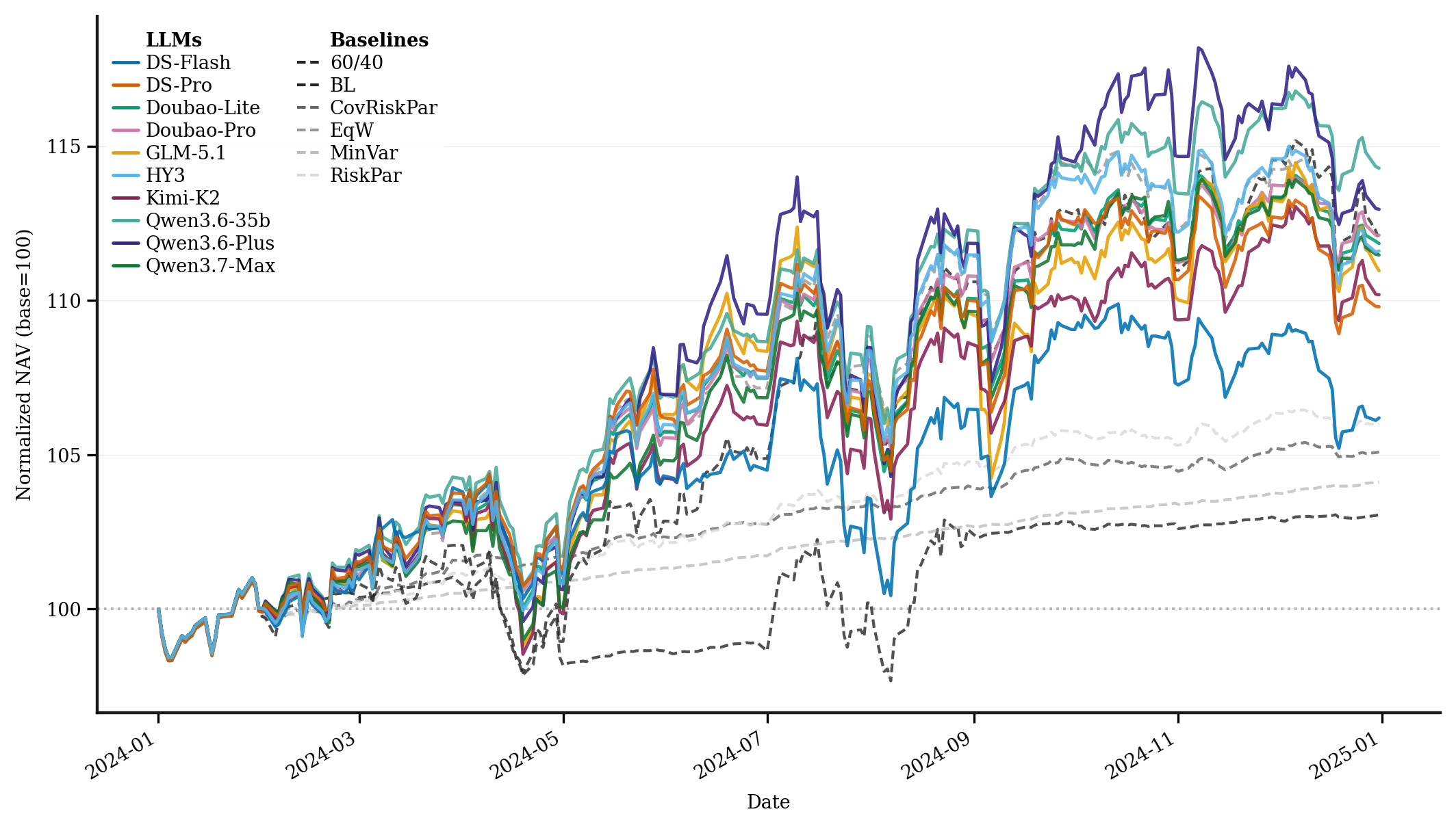
NAV trajectory, balanced

Portfolio NAV trajectories (2024). Shaded band = range across all LLMs; dashed lines = classical baselines.

Stress Regime Results

πŸ”‘ Key Finding Normal-period CEPS rankings do not predict stress survival. Models with strong normal-period CEPS rankings can collapse under historical stress, and the correlation between normal and stress-period scores is weak. Ranking models by calm-market performance alone is insufficient and potentially misleading for real-world deployment. Benchmarks that evaluate only under i.i.d. market conditions systematically overestimate model robustness.

More troubling still, 6 of 10 LLMs fail the Conservative stress gate, all during the 2022 Crypto Collapse. These models satisfy every allocation constraint (equity/crypto caps, bond/cash floors, drawdown/VaR limits) yet still suffer double-digit drawdowns. Small, compliant crypto exposures amplify into portfolio-level losses because the models fail to anticipate cross-asset contagion. Checking procedural boxes does not guarantee outcome-level safety. Stress-regime evaluation is not optional, as it is the only layer that reveals which models are genuinely safe.

The stress gate is defined as follows: a model passes for a given profile if its maximum drawdown across all three historical stress regimes stays within the profile's tolerance. The images below show aggregate stress performance across all models and profiles.

Max drawdown across three stress regimes (worst case, all profiles). Six of ten LLMs fail Conservative.

Normal-period vs. stress-period CEPS (2022, Conservative). High normal scores do not predict stress survival.

Takeaway: Stress-regime evaluation is the only layer that reveals which models are genuinely safe for deployment; normal-period benchmarks alone systematically overestimate robustness.

Static QA Evaluation Results

The rank dissociation above raises a natural question: where do different models excel or struggle within the QA layer itself? The table below breaks down per-template accuracy, revealing sharp divergence between formula-driven tasks (T4, T5) and judgment-driven ones (T1, T2, T6, T7).

Per-template accuracy (full & restricted covariance conditions), formula vs. judgment averages, and accuracy by market regime. Bold = column best. Pink rows = Mean < 0.65.

Model Per-Template (Full) Mean Restricted Task Type Market Regime
T1T2T3T4T5T6T7 T4rT5r FJ BullBearSide.
DeepSeek-V4-Flash.520.843.9451.00.932.652.843.819.975.860.966.715.827.823.812
Qwen3.7-Max.500.859.9511.00.954.724.742.8191.00.990.977.706.814.863.810
DeepSeek-V4-Pro.520.837.9631.00.992.652.760.8181.00.660.996.692.844.846.802
Doubao-Seed-2.0-Lite.460.798.957.956.897.810.747.804.961.940.927.704.780.846.806
Doubao-Seed-2.0-Pro.440.847.963.991.912.824.530.787.979.923.952.660.764.806.792
Qwen3.6-Plus.440.858.9681.00.804.640.768.7831.00.810.902.677.799.801.771
GLM-5.1.440.855.9641.00.421.882.738.7571.00.531.711.729.778.765.746
Qwen3.6-35B-A3B.460.808.9611.00.230.564.763.6841.00.320.615.649.714.729.662
Hunyuan3-Preview.460.386.336.975.958.468.783.624.982.974.967.524.664.663.597
Kimi-K2.6.420.422.493.956.280.684.320.511.978.710.618.462.556.531.487

F = mean(T4,T5) formula-driven; J = mean(T1,T2,T6,T7) judgment-driven. Restricted (T4r, T5r) withholds the covariance matrix: 7 of 10 models perform better without it, confirming format matching rather than genuine numerical reasoning.

QA–Pipeline Rank Dissociation

πŸ”‘ Key Finding QA performance does not imply pipeline competence. The Spearman rank correlation between QA accuracy and pipeline CEPS is ρ = βˆ’0.32. GLM-5.1 ranks 7th in QA yet 1st in CEPS; Kimi-K2.6 ranks last in QA yet 3rd in CEPS. Doubao-Seed-2.0-Lite ranks 4th in QA but last in CEPS, answering static questions correctly yet failing to translate that knowledge into executable portfolio decisions. QA measures isolated factual recall; CEPS measures sustained reasoning across five causally dependent stages. The dissociation is driven by S4 execution fidelity: models that ace formula-driven tasks (T4/T5) often collapse when translating signals into actual orders.

Model QA Mean QA Rank CEPSbal CEPS Rank Ξ”Rank
DeepSeek-V4-Flash.8191.4632βˆ’1
Qwen3.7-Max.8192.3848βˆ’6
DeepSeek-V4-Pro.8183.3659βˆ’6
Doubao-Seed-2.0-Lite.8044.35710βˆ’6
Doubao-Seed-2.0-Pro.7875.4056βˆ’1
Qwen3.6-Plus.7836.4264+2
GLM-5.1.7577.4701+6
Qwen3.6-35B-A3B.6848.4245+3
Hunyuan3-Preview.6249.3897+2
Kimi-K2.6.51110.4343+7

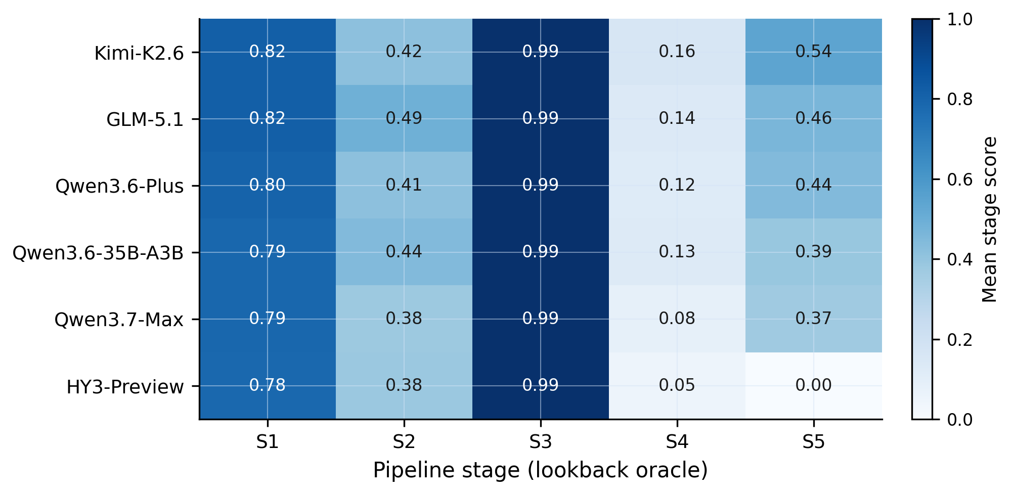
S2 (signal) vs. S4 (execution). Hunyuan3-Preview leads S2 yet collapses in S4: strong signals, no execution.

Profile Alignment Score (PAS) per model. GLM-5.1 applies a nearly identical allocation regardless of risk profile (Οƒ = 0.014).